- On sale!
- Out of stock
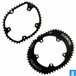
O.Symetric Oval Chainring 130BCD 5-arms
O.Symetric oval chainrings give you 10% more power and more acceleration, and takes 10% less energy and lactate
- Fast shipping
- Not good, money back guarantee
- Safe and secure ordering and payment
- Ordered before 15:30, shipped today.
- Expert advice
- 8.8 with 1019 reviews
Product Info
This outer oval chainring of O.symetric is reco mmended for time trial / race / recreation
The benefits of O.symetric oval chainrings
The oval chainrings of O.symetric are being used by Chris Froome. The reason that no more continental riders are using the oval chainrings of O.symetric is a matter of sponsor interests. But there are more reasons why you may not want to choose de oval chainrings of O.symetric.
- +10% power
- +10% acceleration
- - 10% lactate production
- Less fatigue
- Natural pedalling / cycling
- Triathlon: the cycle to run transition is easier
For most of the bikes is a mounting kit a must, the derailleur should move up a bit.
Why does you need to get oval chainrings of O.symetric
The oval chainrings of O.symetric are fully optimized; which means; the engineers of O.symetric looked exactly how much power the rider supplies in the crank position, the ovality of the chainring is exactly adjusted at the right moment. Besides to that is this concept has been tested in daily use for many years instead of purely ‘drawing table studies’.
With the oval chainrings of O.symetric you’ll know for sure you’ll get the best results of your pedalling and by using more muscles it has proven that the acidification (lactate production) will come later or won’t come at all.
So cycle harder with less lactate, that’s a big reason many riders have chosen the oval chainrings of O.symetric.
The negative sides of O.symetric oval chainrings
Because of the oval chainrings of O.symetric are the biggest possible oval chainrings on the market which are used on a system that is normally used for round chainrings there are some negative sides to the oval chainrings of O.symetric.
- If you’re not cycling ‘pedal to the metal’, you surely can feel the point of change from large to small oval (position ‘five to six’). This could feel annoying.
- Because of you are riding on a system that is built for round chainrings, it is possible that you lose some gears. The so-called “crooked switch” is not possible anymore, in other words: when you’re cycling on the biggest front chainring it is not possible to use the biggest back gear. Also small to small is not possible anymore.
- If you want to use all your gears and want 100% optimal gearing you can choose for the oval chainrings of Rotor (Q-rings). With the oval chainrings of O.symetric you maybe should hold the gear-adjuster a bit longer for a smooth gearchange.
The above ‘negative’ sides of O.symetric chainrings are not meant to scare. Nowadays there are thousands of cyclist who are using the oval chainrings of O.symetric. But we want to be sure you know these negative sides of O.symetric so you can make a proper decision when choosing oval chainrings. We want to get rid of all the bad online stories about the oval chainrings.
When you’re properly informed about the chainrings and thereby make the right choices will everybody cycle better and faster with oval chainrings.
Beneeth tekst from research by Gilbert Storm and Lievin Malfait. See also attached PDF.
Comparative biomechanical study of circular and non-circular chainrings
for endurance cycling at constant speed.
L. Malfait, M.Mech.Eng., G. Storme, M.Sc.Mech.Eng.,
M. Derdeyn, M.Sc.Mech.Eng & Appl.Math.
Abstract – Non-circular chainrings have been available in cycling since the 1890’s. More
recently, Shimano’s Biopace disaster has spoiled the market for oval chainrings. The Harmonic
(1994) was re-launched in 2004 under the brand name O.symetric with some important
successes in professional cycling. In 2005, the Q-Ring (Rotor) entered the cycling scene.
However, non-circular chainwheels have not yet conquered the cycling world. There are many
reasons for this: the conservative world of cycling, the suffocating market domination of an
important manufacturer (and sponsor) of circular chainrings, the difficult bio-dynamics not
understood by users and last but not least, it is not easy to measure and to prove the advantages
of non-circular versus circular. Any reasonable non-circular chainwheel has about 50% chance
of being better than the circular shape. The only question is: what is the optimum shape and
how large can the difference be? The objective of this paper is to compare different chainring
designs. Relying on a mathematical model a biomechanical comparison was made between
circular and non-circular chainrings. The results of the study indicate clearly that (Criterion 1)
for equal crank power for both circular and non-circular chainwheels, the peak joint power
loads can be influenced favourably by using non-circular designs. For equal joint moments
(Criterion 2) for both circular and non-circular designs, the model calculates differences in total
crank power and differences in peak joint power loads. Results for both criteria are mostly
concurrent. The analysis also indicates that shape as well as ovality, but also orientation of the
crank relative to the chainring are important parameters for optimum design. It was found that
some non-circular shapes are clearly better than other designs. The mathematical model can
also be used as a tool for design optimization. Besides the commercial available non-circular
chainrings, some ‘academic’ non-circular profiles were investigated.
Release 2 differs from the previous publication by the use of the MATLAB® software package
for the mathematical model in stead of programs developed in Pascal. Conclusions in release 2
completely confirm the findings from the first release, although with more moderate crank
power efficiency gains. In release 2, result tables are replaced by graphs.
1. Introduction
In cycling, the bicycle-rider system can be modelled as a planar five-bar linkage.
See figure 1: Five bar linkage model of the bicycle-rider system.
The links are: the thigh, the shank, the foot, the crank and the linkage crank axiship
joint.
The five pivot points are: the crank axis, the pedal spindle, the ankle joint, the
knee joint and the hip joint.
Two pivot points are considered as fixed: the crank axis and the hip joint.
See among others Redfield and Hull, Journal of Biodynamics, vol 19-1986a,
pages 317-329.
3
Knee
Hip
Thigh
Shank
Foot
Cr ank
Ankle
Pedal
axis Crank axis
footangle
Crankangle
seat - t ube angle
Figure 1: Five bar linkage model of the bicycle-rider system.
For a five-bar linkage, two kinematic variables are necessary to uniquely specify
the linkage motion. Then the entire system is kinematically defined.
Usually the two kinematic variables are the crank angle and the pedal angle.
Hull et al experimentally measured the relationship between the crank angle and
the angle of the pedal. They expressed the pedal angle (= angle of the foot) as a
function of the crank angle.
A relatively accurate representation of this function is a sine function of the
form
Pedal angle () = A1 + A2 * sin (a + A3)
where a is the crank angle
and A1, A2 and A3 are constants experimentally determined.
Using the work of Bolourchi and Hull, we valued
A1 = 20.76°
A2 = 22.00°
A3 = 190.00°
4
Additional information and input data are to be specified:
- Position of the hip axis versus the crank axis (defined by the seat height and
the seat tube angle).
- Length of the bars: crank arm, foot, shank, thigh and the linkage crank axiship
joint.
- Relative position of the centre of gravity of the foot, shank and thigh versus
their pivot points. (*)
- Mass of foot, shank and thigh. (*)
- Moments of inertia of foot, shank and thigh. (*)
- Crank angular velocity.
(*) Values of the anthropometric parameters were estimated using the work of
Dempster, Whitsett and Dapena.
This study assumes a cadence of 90 crank revolutions per minute. Hence cycle
time is 0.667 sec.
This pedalling rate is generally accepted as being optimal (Hull et al) and
preferred by trained endurance cyclists.
The research also assumes a constant speed of the bicycle, which means a
constant chain linear velocity.
As a consequence a circular chainring has a constant angular velocity of the
crank throughout one revolution.
Non-circular chainrings have variations in angular crank velocity during one
crank cycle: this means, the crank angular velocity is a function of time.
The relation ‘crank angular velocity as a function of time’ for non-circular
chainrings must be known and will be investigated later.
The assumption is made that the forces, developed in the muscles of the lower
limbs, are directly related to the moments in the joints (‘joint-torques’): ankle,
knee and hip moments respectively.
Further in this paper, a method of calculation will be developed and presented
which enables determination of the moments (‘torques’) and power in the joints
as a function of the cycle-time.
2. Moments in the joints.
In order to develop a well-defined force on the pedal, the related muscles of the
joints have to develop in each of the joints a well-defined joint moment (joint
torque).
The force on the pedal (pedal force vector) varies in magnitude and in
orientation as a function of the crank angle.
5
By means of a pedal dynamometer, the normal and tangential components of the
pedal force were measured and registered as a function of time.
These measurements were executed at constant (steady state) crank cadence (90
rpm) and at constant power level (200 W), see figure 2.
Pedal Forces
-250
-200
-150
-100
-50
0
50
0
72
144
216
288
360
Crank Angle
Forces (N)
Tangential Force
Normal Force
Figure 2: Measured tangential and normal pedal forces (Hull et al)
Given the measured normal and tangential pedal forces and taking into account
the known relationship of the pedal angle as a function of the crank angle, the
normal and tangential crank force as a function of the crank angle can be
calculated.
The tangential crank force delivers the crank moment and consequently the
crank power.
See figure 3: Relationship between tangential and normal pedal forces and crank
forces.
Using vector decomposition techniques the force vector on the pedal can be
decomposed into horizontal (X) and vertical (Y) direction respectively:
Fx: denotes the horizontal pedal force component
Fy: denotes the vertical pedal force component
Both pedal force components, together with the dynamic forces and the
moments of the limbs are used to calculate the joint moments.
See figure 4: Pedal force vector decomposition: tangential and normal, Fx, Fy.
6
Foot Pedal
Cr ank Normal
crankf or ce
Tangent .
Crankforce
Pedal force
Tangent .
Pedalf or ce
Normal
Pedalforce
Figure 3: Relationship between tangential and normal pedal forces
Relationship between tangential and normal crank forces
+X
+Y
Fy
Fx Pedal Foot
Crank
Normal
Pedalforce
Tangent .
Pedal f or ce
Figure 4: Pedal force vector decomposition: tangential and normal, Fx, Fy.
7
By means of inverse dynamics the joint forces and the joint moments were
calculated, ref. figure 5.
Fhy
Fhx
X6,Y6
Xcgd,Ycgd
-mdg
X5,Y5
-Mk
-Fkx
-Fky
Mh
X5,Y5
Fky
Fkx
Mk
Xcgb,Ycgb
-mbg
-Fax X4,Y4
-Fay
-Ma
Fay
Fax
Ma
Xcgv,Ycgv X4,Y4
-mfg
Pfh
Pfv
X2,Y2
Hip
Thigh
Knee
Knee
Ankle
Ankle
Pedal axis
Shank
Foot
Figure 5: Free body diagrams of each link: balances of forces and moments.
Pfv = -Fy
Pfh = -Fx
8
The position data of each of the joints were calculated as a function of time.
Given the calculated position data of each of the limbs (links):
by taking the first derivative
- the linear velocity of the centre of gravity in X and Y
- the angular velocity of the limbs
- the angular velocity of the joints
were calculated.
by taking the second derivative
- the linear accelerations in X and Y
- the angular accelerations
were calculated.
From the free-body diagram (see figure 5) the reaction forces in the joints and
the joint moments can be calculated for the ankle, the knee and finally for the
hip.
For the foot with ankle joint:
Fax = mf * aXcgf – Pfh
Fay = mf * aYcgf – Pfv + mf * g
Ma = If * afootangle – Pfv * (X4 – X2) + Pfh * (Y4 – Y2)
– Fay * (X4 – Xcgf) + Fax * (Y4 - Ycgf)
Nomenclature:
Ma = ankle moment.
If = moment of inertia of the foot about the centre of gravity.
afootangle = angular acceleration of the foot.
Pfv = reaction force at the pedal, vertical component.
Pfh = reaction force at the pedal, horizontal component.
X2, Y2 = coordinates of pedal spindle.
X4, Y4 = coordinates of ankle axis.
Xcgf, Ycgf = coordinates of the centre of gravity of the foot.
Fax = force at the ankle joint, X component.
Fay = force at the ankle joint, Y component.
mf = mass of the foot.
aXcgf = linear acceleration of the centre of gravity of the foot, X component.
aYcgf = linear acceleration of the centre of gravity of the foot, Y component.
g = acceleration of gravity (9.81 m/s²)
9
Similar equations are defined for the shank with the knee joint and for the thigh
with the hip joint.
The total joint moments given in the equations above are determined by the
static forces and dynamic forces and the respective moments.
Figure 6 shows the schematic of this partitioning providing a valuable insight
into the dynamics of the pedalling process.
Joint power = Joint moment * Joint angular velocity
Joint angular velocity is a function of crank angular velocity.
As a consequence, for a given bar geometry, given anthropometric data and a
given pedalling rate, the dynamic forces (-moments) can be influenced by
varying the crank angular velocity.
The variation of the crank angular velocity changes the dynamic joint moments,
via the dynamic forces and –moments of the leg segments (limbs). These
10
changes affects the instantaneous total joint moment and the instantaneous total
joint power.
This insight leads to the conclusion that changing the crank angular
velocity gives the opportunity to introduce possible improvements to the
drive mechanism of the bicycle.
Taking a constant pedalling rate for both means that:
- the circular chainring has a constant crank angular velocity
- the non-circular chainring has a varying crank angular velocity, which is
defined by the geometry of the chainring.
3. Method to calculate the crank angular velocity and crank angular
acceleration for any chainring geometry.
The chainring geometry has to meet the following conditions:
1. The contour of the pitch-polygon (pitch-curve) must be equal to n times
the pitch of the chain, whereof n equals the number of chainring teeth.
2. Each side of the pitch-polygon must be exactly equal to the pitch of the
chain.
3. The chainring geometry must be convex; this means no concave sections
are allowed.
4. Point-symmetry for the pitch-curve is a minimum condition.
Constructive limitations may also arise because of the front derailleur: the ratio
major axis versus minor axis (ovality) of a non-circular chainring has to be kept
within certain limits.
In order to define the crank angular velocity as a function of time for a noncircular
chainring, the combination chainring-chain must be considered.
This remains also the case even when the pitch-curve is mathematically defined
e.g. for an ellipse.
The procedure to follow is visualised in figure 7.
Keeping the ‘working chain length’ constant, the successive positions of the
chainring were drawn (using AutoCAD software), each time corresponding with
one tooth rotation of the sprocket. One tooth rotation also equals one time unit
(constant speed of the bicycle is assumed).
In case the curving of the chainring is not constant (non-circular), a deviation
versus the theoretical angle of rotation was measured (a kind of ‘interference’).
Applying this method for each chainring tooth, a matrix with crank angle
positions and corresponding time can be created.
11
Figure 7: How to measure the crank angle per unit of time.
By means of curve-fitting techniques (polynomial regression) the most optimal
mathematical expression of the crank angle as a function of time is calculated.
In general, a nine degree polynomial of the form
Y = A0 + A1*X + A2 *X2 + A3 *X3 + …… + AN *XN
with N = 9
fits closely to the data (correlation > 0.9999).
By taking the first derivative of the equation, with respect to time, the
relationship “crank angular velocity as a function of time” is determined.
By taking the second derivative with respect to time, the relationship ‘crank
angular acceleration as a function of time’ is determined.
4. Criteria of bio-mechanical comparison circular with non-circular
chainrings.
The mathematical model was programmed using MATLAB® software. The
MATLAB® symbolic math toolbox generates and calculates all the necessary
first and second derivates.
The ten coefficients of the polynomial equation of the crank angle as a function
of time are used as input data.
Antropometric, geometric, and other data are constants stored in the
MATLAB® files and are adaptable if needed.
The circular chainring is considered as being the reference.
12
Data of standard pedal forces as a function of time are applied in case of the
circular chainring.
The pedal force profile measured by Hull et al is used (see figure 2). This
approach is acceptable for a comparative study.
All chainrings considered in the study are “normalised” in AutoCAD to 50 teeth.
Given the above-mentioned data, by means of MATLAB®, the mathematical
model calculates the moments and the power as well as further outputs.
All important output data are represented in graphs, using MATLAB® graphic
tools.
Criterion 1:
Given the same instantaneous crank-power development throughout the full
crank cycle for both circular and non-circular chainrings,
the development of the joint-power was calculated for both circular and noncircular
designs. Calculations were executed for the knee and the hip joint.
During the first part of the cycle, where the joint angular velocity is positive, the
extensor muscles of the joints are the main drivers. For the hip this is mainly the
Gluteus Maximus and for the knee primarily the Rectus Femoris and the Vastii.
During the second part of the cycle, where the joint angular velocity is negative,
the flexor muscles of the joints are the main drivers. For the hip this is mainly
the Rectus Femoris and for the knee primarily the Gastrocnemius, the Biceps
Femoris and the Hamstrings.
Approach:
In a first run,
the MATLAB® program calculates the positions, the velocities, the
accelerations, the total joint moments, the total joint power and the crank power
of the circular chainring.
The pedal reaction forces in the X and Y directions were calculated using the
normal and tangential pedal forces measured by Hull et al (see figure 2).
Time was declared as a symbolic variable, so all subsequent equations were
evaluated as a function of time.
A graph of the knee power and the hip power development as a function of time
was prepared.
13
In a second run,
MATLAB® calculates the crank angular velocity of the non-circular chainring
being the first derivate of the crank angle versus time.
The crank power as a function of time, taken over from the first run (circular
chainring), was now used as input.
From this, the pedal reaction forces in the X and Y directions were deduced,
assuming that these reaction forces relate to each other in the same way as the X
and Y components of the circular chainring do.
Knee power and hip power versus time were now recalculated.
Plots of knee power and hip power versus time for both the circular and non
circular chainring, are presented.
Criterion 2:
Comparison of the total crank power over the full crank cycle taking into
account identical development of the instantaneous joint-moments for both,
circular and non-circular chainring..
Approach:
In a first run,
the MATLAB® program calculates the positions, velocities, accelerations, total
joint-moments, total joint power and crank power of the circular chainring.
Time is declared as a symbolic variable, so all subsequent equations are
evaluated as a function of time.
A graph of the crank power as function of time is prepared.
In a second run,
MATLAB® calculates the crank angular velocity of the non-circular chainring,
being the first derivate of the crank angle versus time.
The joint-moments as function of time, taken over from the first run are now
used to recalculate the X and Y components of the crank force. Here from, crank
power versus time is calculated and a plot of crank power versus time is
presented.
The graphs are clearly showing the differences in crank power development
between the circular and the compared non-circular chainring.
A MATLAB® tool allows to calculate and to display the mean value of the
crank power over one full cycle for one pedal, for both the circular and the non
circular chainring.
14
5. Non-circular chainring types
Convention: 1. Crank angle
* crank arm vertical equals 0°,
arbitrary defined as being “Top-Dead-Centre” (T.D.C.)
*rotation: counter clockwise
*crank angle is being measured from T.D.C
( = crank arm vertical), counter clockwise, to major axis.
2. Ovality (‘e’ in the figures): ratio of major axis to minor axis
• O.symetric-Harmonic
-designed: 1993
-inventors: J.L. Talo & M. Sassi, France
-ovality: 1.215
-geometry: see figure 8
-symmetry: point symmetric (bi-radial)
-chainring radius proportional with variation of crank torque
-angle major axis versus crank arm: 78 ° (major axis assumed to be the
middle of the circle segment of the oval);
-radial oriented chainring teeth
-commercialised
Figure 8: O.symetric-Harmonic
• Hull oval
-designed: 1991
-inventor: prof M.L. Hull, Univ California, Davis, USA
-ovality: 1.55
-geometry: see figure 9
-symmetry: point symmetric (bi-radial)
15
-theoretical shape to eliminate “internal work”
-angle major axis vs crank arm: 90°
-not commercialised
Figure 9: Hull oval
• Rasmussen oval
-designed: 2006
-inventor: prof John Rasmussen, Univ of Aalburg, Denmark
-ovality: 1.30
-geometry: ellipse-like, see figure 10
-symmetry: bi-axis symmetric
-designed to minimize maximum muscle activation
-angle major axis vs crank arm: 72°
-not commercialised
Figure 10: Rasmussen oval
16
• Q-Ring (Rotor)
-designed: 2005
-inventor: Pablo Carrasco, Rotorbike, Spain
-ovality: 1.10
-geometry: modified ellipse (circle arcs at extremities of major axis), see
figure 11
-symmetry: bi-axis symmetric
-designed to minimize time spent in the dead spots and to maximize the
benefit of the power stroke
-angle major axis vs crank arm: adjustable, advised 70°-75°
-commercialised
Figure 11: Q-Ring
• Biopace oval
- designed: 1983
-inventor: Shimano, Japan (Prof. Okajima)
-ovality: 1.04 (earlier makes 1.09, 1.17…)
-geometry: skewed ellipse with major and minor axes not perpendicular,
see figure 12
-symmetry: point symmetric
-designed to take advantage of leg inertia
-angle major axis vs crank arm: -8° (crank arm approximately parallel to
major axis)
-commercialised
17
Figure 12: Biopace
• OVUM ellipse
- designed: before 1980 (?)
-inventor: ?
-ovality: different types, 1.18 and 1.235
-geometry: ellipse, see figure 13
-symmetry: bi-axis symmetric
-designed to reduce negative effects of dead spots
-angle major axis vs crank arm: 90° ( also types with adjustable crank
orientation)
-commercialised
Figure 13: OVUM ellipse
18
• Ogival oval
- designed: 1993
-inventor: Bernard Rosset, France
-ovality: 1.235
-geometry: intersection of 2 circle arcs with circle centres on minor axis,
see figure 14
-symmetry: bi-axis symmetric
-designed to reduce negative effects of dead spots and facilitate climbing
-angle major axis vs crank arm: 54°
-commercialised
Figure 14: Ogival
• Polchlopek oval
- designed: 1970 (?)
-inventor: Edmond Polchlopek, France
-ovality: 1.214
-geometry: 2 semicircles joined by 2 bridges of 3 ‘flat’ teeth, see figure 15
-symmetry: bi-axis symmetric
-designed to reduce negative effects of dead spots
- angle major axis vs crank arm: 102°
-commercialised
19
Figure 15: Polchlopek oval
• LM-Super oval
-designed: 2009
-inventor: Lievin Malfait
-ovality: 1.31
-geometry: see figure 16
-symmetry: point symmetric (bi-radial)
-chainring reflects polar plot of crank torque throughout one crank cycle
-angle major axis versus crank arm: adjustable from 78° to 118° in 5
positions (major axis assumed to be the middle of the circle segment of
the oval);
-the ‘flat teeth segment’ and the “circle segment” are bridged by an
Archimedean spiral segment.
-chainring teeth perpendicular on the pitch-curve.
-not commercialised
20
Figure 16: LM-Super oval
6. Biomechanical results
The properties and performances of the different non-circular chainrings
examined in this paper, are displayed in the pictures and graphs below.
At the top of each page the pictures show the shape, the ovality and two
different crank orientations of the chainring involved: on the left, the crank
positioning proposed by the inventor or designer and, on the right, the optimal
orientation calculated by this study.
In the middle of the page, the performances with respect to criterion 2 are
plotted (crank power development at equal joint moments, circular and noncircular).
The mean crank power of the non-circular chainring, calculated by MATLAB®,
is plotted as a dash-dotted red line. A data tip indicates the value of the mean
crank power of the non-circular.
The mean crank power of the circular chainring, also calculated by MATLAB®,
is 104 W in all cases and is mentioned on the graphs.
The ratio between the mean non-circular crank power and the mean circular
crank power is a measure for the efficiency gain of the non-circular chainring,
compared to a circular one.
21
As an example: a ratio of 1.025 means that, at equal joint moments, the mean
crank power of the non-circular chainring is 2.5 % superior versus the mean
crank power of the circular, which is favourable.
At the bottom of the page, the graphs show the performances with respect to
criterion 1 (development of knee and hip power at equal crank power, circular
and non-circular).
Data tips indicate the knee peak power (extensor muscles) for both the circular
and non-circular chainring.
The ratio between the knee peak power (extensor muscles) of the non-circular
chainring versus circular is a measure of the efficiency with respect to the knee
joint peak load (extensor muscles).
As an example: a ratio of 0.94 (or 94%) means that, at equal crank power, the
peak knee power (extensor muscles) is 6% inferior with a non-circular chainring
compared to a circular one, which is favourable.
In cycling, the knee extensor muscles are assumed to be of major importance.
Muscular fatigue and (knee) injuries primarily are caused by peak joint loads.
Hence, comparing the knee peak power generated by the knee extensor muscles
is useful and is a well-founded basis to compare and to judge the performances
of non-circular chainrings.
Information about the development of the peak power loads in the knee flexor
muscles, in the hip extensor muscles and in the hip flexor muscles, for both
circular and non-circular chainring, can be found by reading out the different
graphs (values are not mentioned in the overview tables).
6.1. Optimal crank orientation
By changing step-by-step the crank angle versus the major axis of the noncircular
chainring we can search for an optimal crank orientation.
An optimal crank position would mean:
-the lowest peak power load in the joints, given the same crank power
development (criterion 1)
-the highest crank power efficiency, combined with the lowest peak power
load in the extensor joint muscles of knee and hip, given the same joint
moments (criterion 2)
for both, circular and non-circular.
22
As an example we study the O.symetric case.
versus circular chainring
Criterion 1 Criterion 2
Angle Major
Axis
versus Crank
Peak Power
Knee
Extensor
Crank Power Peak Power
Knee
Extensor
Peak Power
Hip
Extensor
78.0° -1.5% vs circ. -0.7% vs circ. -1.8% vs circ. +4.6% vs circ.
109.6° -7.9% +2.4% -10.0% +15.1%
117.0° -7.5% +2.5% -10.0% +16.2%
124.3° -6.5% +2.9% -9.9% +15.4%
128.0° -4.9% +2.9% -7.6% +14.0%
132.0° -3.2% +2.7% -6.0% +18.0%
We notice the same trend for all the investigated chainring designs.
As a general rule we may conclude that the optimal crank orientation is located
in the zone from 110° up to 120°, angle between major axis of the non-circular
chainring and the crank, measured counterclockwise.
In case the crank is optimal oriented and the major axis of the non-circular
chainring is vertical then we see the crank arm roughly perpendicular on the seat
tube direction (“rule of thumb”).
Above mentioned figures are applicable for a seat tube angle of about 73°.
The optimal crank orientation is a function of the bicycle geometrie and the
anthropometric parameters of the rider.
Simulations with a seat tube angle of e.g. 78° (time trial bike) learn that the
optimal zone is located in the range between 105° and 115°.
23
6.2. Graphs
Biopace Original -8.2°
0 0.1 0.2 0.3 0.4 0.5 0.6 0.7
−100
−50
0
50
100
150
200
250
300
350
400
X: 0
Y: 103.8
Time (Sec)
Crank Power ( W )
Crank Power − Circular vs biopace Orig., at equal Joint Moments −− 90 Rpm
Angle Major axis vs Crank : −8.2 °−− Ovality : 1.04
Crank Pow. Circular
Crank Pow. Non−Circ.
mean Non−Circ.
Mean Circ:
104
0 0.1 0.2 0.3 0.4 0.5 0.6 0.7
−200
−100
0
100
200
300
X: 0.1067
Y: 277.5
X: 0.12
Y: 280.6
Time (Sec)
Knee & Hip Power ( W )
Knee & Hip power Circular vs biopace Orig., at equal Crank Power −− 90 Rpm
Angle Major axis vs Crank : −8.2 °−− Ovality1.1
Hip Circular
Knee Circular
Hip Non−Circ
Knee Non−Circ
Biopace Orig./Circ:
101 %
24
Hull Original 90° Hull Optimal 107°
0 0.1 0.2 0.3 0.4 0.5 0.6 0.7
−100
−50
0
50
100
150
200
250
300
350
400
X: 0
Y: 104.6
Time (Sec)
Crank Power ( W )
Crank Power − Circular vs Hull Orig., at equal Joint Moments −− 90 Trm
Angle Major axis vs Crank : 90 °−− Ovality : 1.55
Crank Pow. Circular
Crank Pow. Non−Circ.
mean Non−Circ.
Mean Circ=
104
0 0.1 0.2 0.3 0.4 0.5 0.6 0.7
−100
−50
0
50
100
150
200
250
300
350
400
X: 0
Y: 107.4
Time (Sec)
Crank Power ( W )
Crank Power − Circular vs Hull + 2T, at equal Joint Moments −− 90 Rpm
Angle Major axis vs Crank : 107.5 °−− Ovality : 1.55
Crank Pow. Circular
Crank Pow. Non−Circ.
mean Non−Circ.
Mean Circ=
104
0 0.1 0.2 0.3 0.4 0.5 0.6 0.7
−200
−150
−100
−50
0
50
100
150
200
250
300
X: 0.12
Y: 277
X: 0.08
Y: 259.1
Time (Sec)
Knee & Hip Power ( W )
Knee & Hip power Circular vs Hull Orig., at equal Crank Power −− 90 Rpm
Angle Major axis vs Crank : 90 °−− Ovality1.55
Hip Circular
Knee Circular
Hip Non−Circ
Knee Non−Circ
Hull Orig/Circ:
94.5
0 0.1 0.2 0.3 0.4 0.5 0.6 0.7
−300
−200
−100
0
100
200
300
X: 0.12
Y: 277
X: 0.1067
Y: 244.8
Time (Sec)
Knee & Hip Power ( W )
Knee & Hip power Circular vs Hull + 2T, at equal Crank Power −− 90 Trm
Angle Major axis vs Crank : 107.5 °−− Ovality1.55
Hip Circular
Knee Circular
Hip Non−Circ
Knee Non−Circ
Hull +2/Circ:
88.2 %
25
Osymetric Original 78° Osymetric 117°
0 0.1 0.2 0.3 0.4 0.5 0.6 0.7
−100
−50
0
50
100
150
200
250
300
350
400
X: 0
Y: 103.3
Time (Sec)
Crank Power ( W )
Crank Power − Circular vs Osymetric original, at equal Joint Power −− 90 Rpm
Angle Major axis vs Crank : 78°
Crank Pow. Circular
Crank Pow. Non−Circ.
mean Non−Circ
mean circ:
104
0 0.1 0.2 0.3 0.4 0.5 0.6 0.7
−100
−50
0
50
100
150
200
250
300
350
400
X: 0
Y: 106.6
Time (Sec)
Crank Power ( W )
Crank Power − Circular vs Osymetric +5T rotated, at equal Joint Moments −− 90 Rpm
Angle Major axis vs Crank : 117°
Crank Pow. Circular
Crank Pow. Non−Circ.
mean Non−Circ
Mean Circ =
104
0 0.1 0.2 0.3 0.4 0.5 0.6 0.7
−200
−150
−100
−50
0
50
100
150
200
250
300
X: 0.12
Y: 277
X: 0.09333
Y: 273.3
Time (Sec)
Knee & Hip Power ( W )
Knee & Hip power Circular vs Osymetric original, at equal Crank Power −− 90 Rpm
Angle Major axis vs Crank : 78°−− Ovality1.215
Hip Circular
Knee Circular
Hip Non−Circ
Knee Non−Circ
Osy Orig/Circ:
98.5 %
0 0.1 0.2 0.3 0.4 0.5 0.6 0.7
−200
−150
−100
−50
0
50
100
150
200
250
300
X: 0.1067
Y: 277.5
X: 0.12
Y: 256.5
Time (Sec)
Knee & Hip Power
Knee & Hip power Circular vs Osymetric+5t at equal Crankpower 90 Rpm
Angle Major axis vs Crank: 117°
Hip circular
Knee circular
Hip Osymetric+5
Knee Osymetric+5
Osy5/Circ:
92.5 %
Osy/Circ:
110 %
26
Ogival Original 54° Ogival Optimal 110.5°
0 0.1 0.2 0.3 0.4 0.5 0.6 0.7
−100
−50
0
50
100
150
200
250
300
350
400
Time (Sec)
Crank Power ( W )
Crank Power − Circular vs Ogival
o
rig, at equal Joint Moments −− 90 Rpm
Angle Major axis vs Crank : 54 °−− Ovality : 1.235
X: 0
Y: 97.3
Crank Pow. Circular
Crank Pow. Non−Circ.
mean Non−Circ.
Mean Circ =
104
0 0.1 0.2 0.3 0.4 0.5 0.6 0.7
−100
−50
0
50
100
150
200
250
300
350
400
X: 0
Y: 104.6
Time (Sec)
Crank Power ( W )
Crank Power − Circular vs Ogival +7T, at equal Joint Moments −− 90 Rpm
Angle Major axis vs Crank : 110.5−− Ovality : 1.235
Crank Pow. Circular
Crank Pow. Non−Circ.
mean Non−Circ.
Mean Circ =
104
0 0.1 0.2 0.3 0.4 0.5 0.6 0.7
−200
−150
−100
−50
0
50
100
150
200
250
300
X: 0.09333
Y: 297
X: 0.1067
Y: 277.5
Time (Sec)
Knee & Hip Power ( W )
Knee & Hip power Circular vs Ogival
o
rig, at equal Crank Power −− 90 Rpm
Angle Major axis vs Crank : 54 °−− Ovality1.235
Hip Circular
Knee Circular
Hip Non−Circ
Knee Non−Circ
Ogival−Orig/Circ.
107 %
0 0.1 0.2 0.3 0.4 0.5 0.6 0.7
−200
−150
−100
−50
0
50
100
150
200
250
300
X: 0.1067
Y: 277.5
X: 0.1067
Y: 259.3
Time (Sec)
Knee & Hip Power ( W )
Knee & Hip power Circular vs Ogival +7T, at equal Crank Power −− 90 Rpm
Angle Major axis vs Crank : 110.5−− Ovality1.235
Hip Circular
Knee Circular
Hip Non−Circ
Knee Non−Circ
Ogival7/Circ:
93.5 %
27
Q-Ring original 74° Q-Ring optimal 107.5°
0 0.1 0.2 0.3 0.4 0.5 0.6 0.7
−100
−50
0
50
100
150
200
250
300
350
400
X: 0
Y: 99.24
Time (Sec)
Crank Power ( W )
Crank Power − Circular vs Q−ring original, at equal Joint Moments −− 90 Rpm
Angle Major axis vs Crank : 74°−− Ovality : 1.1
Crank Pow. Circular
Crank Pow. Non−Circ.
mean Non−Circ.
mean Circ:
104
0 0.1 0.2 0.3 0.4 0.5 0.6 0.7
−100
−50
0
50
100
150
200
250
300
350
400
X: 0
Y: 104.2
Time (Sec)
Crank Power ( W )
Crank Power − Circular vs Q−ring +4T rotated, at equal Joint Moments −− 90 Rpm
Angle Major axis vs Crank : 107.5°−− Ovality : 1.1
Crank Pow. Circular
Crank Pow. Non−Circ.
mean Non−Circ.
mean Circ. =
104
0 0.1 0.2 0.3 0.4 0.5 0.6 0.7
−200
−150
−100
−50
0
50
100
150
200
250
300
X: 0.09333
Y: 281.4
X: 0.12
Y: 277
Time (Sec)
Knee & Hip Power
Knee & Hip power Circular vs Q−ring origineel, at equal Crank Power −− 90 Rpm
Angle Major axis vs Crank : 74° −− Ovality: 1.10
Hip Circular
Knee Circular
Hip Qring Orig
Knee Qring Orig
Qring−orig/Circ
101.5 %
0 0.1 0.2 0.3 0.4 0.5 0.6 0.7
−200
−100
0
100
200
300
X: 0.1067
Y: 277.5
X: 0.1067
Y: 268.9
Time (Sec)
Knee & Hip Power ( W )
Knee & Hip power Circular vs Q−ring +4T rotated, at equal Crank Power −− 90 Rpm
Angle Major axis vs Crank : 107.5° −− Ovality: 1.10
Hip Circular
Knee Circular
Hip Non−Circ
Knee Non−Circ
Qring+4/Circ:
97 %
28
Ovum-118 Original 90° Ovum 118 Optimal 106°
0 0.1 0.2 0.3 0.4 0.5 0.6 0.7
−100
−50
0
50
100
150
200
250
300
350
400
X: 0
Y: 103.8
Time (Sec)
Crank Power ( W )
Crank Power − Circular vs Ovum 1.18 Orig., at equal Joint Moments −− 90 Rpm
Angle Major axis vs Crank : 90°−− Ovality : 1.18
Crank Pow. Circular
Crank Pow. Non−Circ.
mean Non−Circ.
0 0.1 0.2 0.3 0.4 0.5 0.6 0.7
−100
−50
0
50
100
150
200
250
300
350
400
X: 0
Y: 105
Time (Sec)
Crank Power ( W )
Crank Power − Circular vs Ovum 118 +2T, at equal Joint Moments −− 90 Rpm
Angle Major axis vs Crank : 105.6−− Ovality : 1.18
Crank Pow. Circular
Crank Pow. Non−Circ.
y mean
Mean Circ. =
104
0 0.1 0.2 0.3 0.4 0.5 0.6 0.7
−200
−100
0
100
200
300
X: 0.1067
Y: 277.5
X: 0.1067
Y: 269.8
Time (Sec)
Knee & Hip Power ( W )
Knee & Hip power Circular vs Ovum 1.18 Orig., at equal Crank Power −− 90 Rpm
Angle Major axis vs Crank : 90°−− Ovality1.18
Hip Circular
Knee Circular
Hip Non−Circ
Ovum118−Orig/Circ: Knee Non−Circ
97 %
0 0.1 0.2 0.3 0.4 0.5 0.6 0.7
−200
−150
−100
−50
0
50
100
150
200
250
300
X: 0.12
Y: 277
X: 0.1067
Y: 262.7
Time (Sec)
Knee & Hip Power ( W )
Knee & Hip power Circular vs Ovum 118 +2T, at equal Crank Power −− 90 Rpm
Angle Major axis vs Crank : 105.6−− Ovality1.18
Hip Circular
Knee Circular
Hip Non−Circ
Knee Non−Circ
Ovum 118+2/Circ
94.5 %
29
Ovum-124 Original 90° Ovum-124 Optimal 106°
0 0.1 0.2 0.3 0.4 0.5 0.6 0.7
−100
−50
0
50
100
150
200
250
300
350
400
X: 0
Y: 103.8
Time (Sec)
Crank Power ( W )
Crank Power − Circular vs Ovum 124 Orig, at equal Joint Moments −− 90 Rpm
Angle Major axis vs Crank : 90 °−− Ovality : 1.24
Crank Pow. Circular
Crank Pow. Non−Circ.
mean Non−Circ.
mean Circ. =
104
0 0.1 0.2 0.3 0.4 0.5 0.6 0.7
−100
−50
0
50
100
150
200
250
300
350
400
X: 0
Y: 105.3
Time (Sec)
Crank Power ( W )
Crank Power − Circular vs Ovum 124 +2T, at equal Joint Moments −− 90 Rpm
Angle Major axis vs Crank : 106 °−− Ovality : 1.24
Crank Pow. Circular
Crank Pow. Non−Circ.
mean Non−Circ.
Mean Circ =
104
0 0.1 0.2 0.3 0.4 0.5 0.6 0.7
−200
−150
−100
−50
0
50
100
150
200
250
300
X: 0.1067
Y: 277.5
X: 0.09333
Y: 268.4
Time (Sec)
Knee & Hip Power ( W )
Knee & Hip power Circular vs Ovum 124 Orig, at equal Crank Power −− 90 Rpm
Angle Major axis vs Crank : 90 °−− Ovality1.24
Hip Circular
Knee Circular
Hip Non−Circ
Knee Non−Circ
Ovum124/Circ
97 %
0 0.1 0.2 0.3 0.4 0.5 0.6 0.7
−200
−150
−100
−50
0
50
100
150
200
250
300
X: 0.1067
Y: 277.5
X: 0.1067
Y: 258.5
Time (Sec)
Knee & Hip power Circular vs Ovum 124 +2T, at equal Crank Power −− 90 Rpm
Angle Major axis vs Crank : 106 °−− Ovality1.24
Hip Circular
Knee Circular
Hip Non−Circ
Knee Non−Circ
Ovum124+2/Circ:
93 %
30
Pochlopek Original 102° Polchlopek optimal 109.5°
0 0.1 0.2 0.3 0.4 0.5 0.6 0.7
−100
−50
0
50
100
150
200
250
300
350
400
X: 0
Y: 105.2
Time (Sec)
Crank Power ( W )
Crank Power − Circular vs Polchlopec Orig., at equal Joint Moments −− 90 Rpm
Angle Major axis vs Crank : 102°−− Ovality : 1.214
Crank Pow. Circular
Crank Pow. Non−Circ.
mean Non−Circ.
Mean circular=
104
0 0.1 0.2 0.3 0.4 0.5 0.6 0.7
−100
−50
0
50
100
150
200
250
300
350
400
X: 0
Y: 105.6
Time (Sec)
Crank Power ( W )
Crank Power − Circular vs Polchlopek+1T, at equal Joint Moments −− 90 Rpm
Angle Major axis vs Crank : 109.5°−− Ovality : 1.214
Crank Pow. Circular
Crank Pow. Non−Circ.
y mean
mean Circ =
104
0 0.1 0.2 0.3 0.4 0.5 0.6 0.7
−200
−150
−100
−50
0
50
100
150
200
250
300
X: 0.1067
Y: 277.5
X: 0.1067
Y: 264.2
Time (Sec)
Knee & Hip Power ( W )
Knee & Hip power Circular vs Polchlopec Orig., at equal Crank Power −− 90 Rpm
Angle Major axis vs Crank : 102° −− Ovality: 1.214
Hip Circular
Knee Circular
Hip Non−Circ
Knee Non−Circ
Polchlopec/Circ
95 %
0 0.1 0.2 0.3 0.4 0.5 0.6 0.7
−200
−150
−100
−50
0
50
100
150
200
250
300
X: 0.1067
Y: 261.3
X: 0.12
Y: 277
Time (Sec)
Knee & Hip Power ( W )
Knee & Hip power Circular vs Polchlopek+1T at equal Crank Power −− 90 Rpm
Angle Major axis vs Crank : 109.5°−− Ovality1.214
Hip Circular
Knee Circular
Hip Non−Circ
Knee Non−Circ
Pol.+1/Circ.=
94.3%
31
Rasmussen Original 73° Rasmussen optimal 113°
0 0.1 0.2 0.3 0.4 0.5 0.6 0.7
−100
−50
0
50
100
150
200
250
300
350
400
X: 0
Y: 101.1
Time (Sec)
Crank Power ( W )
Crank Power − Circular vs Rasmussen Orig., at equal Joint Moments −− 90 Rpm
Angle Major axis vs Crank : 72°−− Ovality : 1.30
Crank Pow. Circular
Crank Pow. Non−Circ.
y mean
Mean Circular=
104
0 0.1 0.2 0.3 0.4 0.5 0.6 0.7
−100
−50
0
50
100
150
200
250
300
350
400
X: 0
Y: 105.7
Time (Sec)
Crank Power ( W )
Crank Power − Circular vs Rasmussen+5, at equal Joint Moments −− 90 Rpm
Angle Major axis vs Crank : 113°−− Ovality : 1.30
Crank Pow. Circular
Crank Pow. Non−Circ.
mean Non−Circ
Mean Circ. =
104
0 0.1 0.2 0.3 0.4 0.5 0.6 0.7
−200
−150
−100
−50
0
50
100
150
200
250
300
X: 0.09333
Y: 286
X: 0.12
Y: 277
Time (Sec)
Knee & Hip Power ( W )
Knee & Hip power Circular vs Rasmussen Orig. at equal Crank Power −− 90 Rpm
Angle Major axis vs Crank : 72°−− Ovality1.30
Hip Circular
Knee Circular
Hip Non−Circ
Knee Non−Circ
Rasm. orig/Circ.
103 %
0 0.1 0.2 0.3 0.4 0.5 0.6 0.7
−300
−200
−100
0
100
200
300
X: 0.1067
Y: 277.5
X: 0.1067
Y: 251.2
Time (Sec)
Knee & Hip Power ( W ) Knee &
Hip power Circular vs Rasmussen+5
at equal Crank Power −− 90 Rpm
Angle Major axis vs Crank : 113°−− Ovality1.30
Hip Circular
Knee Circular
Hip Non−Circ
Knee Non−Circ
rasm+5/Circ=
90.5 %
32
LM-Super - Original 107° LM-Super – Optimal 114.5°
0 0.1 0.2 0.3 0.4 0.5 0.6 0.7
−100
−50
0
50
100
150
200
250
300
350
400
X: 0
Y: 106.5
Time (Sec)
Crank Power ( W )
Crank Power − Circular vs Optimal, at equal Joint Moments −− 90 Rpm
Angle Major axis vs Crank : 107°−− Ovality : 1.31
Crank Pow. Circular
Crank Pow. Non−Circ.
mean Non Circ.
mean Circular =
104
0 0.1 0.2 0.3 0.4 0.5 0.6 0.7
−100
−50
0
50
100
150
200
250
300
350
400
X: 0
Y: 106.8
Time (Sec)
Crank Power ( W )
Crank Power − Circular vs Optimal1, at equal Joint Moments −− 90 Rpm
Angle Major axis vs Crank : 114.5°−− Ovality : 1.31
crank Pow Circ.
Crank Pow Non−Circ.
mean Non−Circ.
Mean Circular =
104
0 0.1 0.2 0.3 0.4 0.5 0.6 0.7
−200
−150
−100
−50
0
50
100
150
200
250
300
X: 0.1067
Y: 277.5
X: 0.1067
Y: 254.7
Time (Sec)
Knee & Hip Power ( W )
Knee & Hip power Circular vs Optimal at equal Crank Power −− 90 Rpm
Angle Major axis vs Crank : 107°−− Ovality1.31
Hip Circular
Knee Circular
Hip Non−Circ
Knee Non−Circ
Optimal−Org/Circ=
92 %
0 0.1 0.2 0.3 0.4 0.5 0.6 0.7
−300
−200
−100
0
100
200
300
X: 0.1067
Y: 277.5
X: 0.1067
Y: 251.9
Time (Sec)
Knee & Hip Power ( W )
Knee & Hip power Circular vs Optimal1 at equal Crank Power −− 90 Rpm
Angle Major axis vs Crank : 114.5°−− Ovality1.31
Hip Circular
Knee Circular
Hip Non−Circ
Knee Non−Circ
Optimal1/Circ:
90.8%
33
6.2. Overview of results
Non Circular
Chainring
shapes
Ratio
Major
versus
Minor
Axis
Angle
Major
Axis
versus
Crank
Peak
Knee Power
Extensors
for same given
Crank Power
% % difference vs
Circular
Crank Power
for same given
Joint Moments
% difference vs
Circular
Biopace 1.04 -8° +1 % -0.2 %
Hull Original 1.55 90° -5.5 % +0.58 %
Hull Optimal 1.55 107.5° -11.8 % +3.3 %
O.symetric Original 1.215 78° -1.5 % -0.67 %
O.symetric Optimal 1.215 117° -7.5 % +2.5 %
Ogival Original 1.235 54° +7 % -6.4 %
Ogival Optimal 1.235 110.5° -6.5 % +0.4 %
Ovum-118 Original 1.18 90° -3 % -0.2 %
Ovum-118 Optimal 1.18 106° -5.5 % +1.0 %
Ovum-124 Original 1.24 90° -3 % -0.2 %
Ovum-124 Optimal 1.24 106° -7 % +1.25 %
Polchlopek Original 1.214 102° -5 % +1.15%
Polchlopek Optimal 1.214 109.5° -5.7 % +1.54 %
Rasmussen Original 1.30 72° +3 % -2.8 %
Rasmussen Optimal 1.30 113° -9.5 % +1.6 %
Q-Ring Original 1.10 74° +1.5 % -4.58 %
Q-Ring Optimal 1.10 107.5° -3 % +0.2 %
LM-Super Original 1.31 107° -8 % +2.4 %
LM-Super Optimal 1.31 114.5° -9.2 % +2.7 %
Ranking
Hull Optimal 1.55 107.5° -11.8 % +3.3 %
LM-Super Optimal 1.31 114.5° -9.2 % +2.7 %
O.symetric Optimal 1.215 117° -7.5 % +2.5 %
Rasmussen Optimal 1.30 113° -9.5 % +1.6 %
Polhlopek Optimal 1.214 109.5° -5.7 % +1.54 %
Ovum-124 Optimal 1.24 106° -7 % +1.25 %
Ovum-118 Optimal 1.18 106° -5.5 % +1.0 %
Ogival Optimal 1.235 110.5° -6.5 % +0.4 %
Q-Ring Optimal 1.10 107.5° -3 % +0.2 %
Biopace 1.04 -8° +1 % -0.2 %
34
7. Concluding remarks
Relying on a mathematical model, a biomechanical comparison was made
between a circular and different non-circular chainring designs.
The mathematical model is partly based on literature study but is also
based on own developments and new insights.
Especially the methodology to accurately measure the crank angle
velocity is new and has, to the authors’ knowledge, not been applied
before. This accurate measuring method is however of paramount
importance with non-circular profiles and is the necessary basis for
reliable input data and hence a guarantee for reliable output results.
Also the choice of the two criteria to compare performances - circular
versus non-circular chainring – is new and has, to the authors’ knowledge,
not been applied before.
The results of this biomechanical study indicate clearly that (criterion 1)
for equal instantaneous crank power for both circular and non-circular, the
peak joint power loads can be influenced favourably or unfavourably by
using non-circular chainring designs.
This is a purely (bio)-mechanical issue.
For equal instantaneous joint moments (criterion 2) for both, circular and
non-circular chainring designs, the model calculates differences in total
crank power efficiency and in peak power loads on the joints.
The results for both criteria are mostly concurrent.
Some non-circular chainring profiles are undeniably better than other
designs and perform clearly better than circular ones, at least according to
the criteria considered in this paper.
An analysis of the test results indicates clearly that three geometric
parameters are important for optimal design of a non-circular chainring,
namely the ovality, the crank orientation and the shape.
A balanced combination of these geometric parameters should result in
the most optimal non-circular chainring compared to circular.
The most optimal solution would mean:
-the lowest peak power load in the joints, given the same crank power
development (criterion 1)
-the highest crank power efficiency, combined with the lowest peak power
load in the extensor joint muscles of knee and hip, given the same joint
moments (criterion 2)
for both circular and non-circular.
35
A first important finding of the study is that a minimum ovality is needed
to be able to yield attractive power efficiency rates. The results also show
that a positive correlation exists between the degree of ovality and the
attainable crank power efficiency percentage compared to circular.
A second interesting conclusion is that for a specific non-circular
chainring, peak power loads on the joints and the crank power efficiency
can be adapted continuously by changing the crank orientation versus the
major axis of the oval.
However, the results of the biomechanical study show clearly that, in
many cases, ‘advantages’ and ‘disadvantages’ are inseparable.
Indeed, by increasing the crank angle versus the major axis,
for criterion 1 and criterion 2, it becomes apparent that:
• peak power load on both knee joint muscle groups, extensors and flexors,
is decreasing, whereby:
peak power load of the extensors decreases to a minimum at
optimal crank angle orientation. This minimum is below
circular chainring peak power load.
peak power load of the flexors is mostly above circular
chainring peak power load.
• peak power load on both hip joint muscle groups, extensors and flexors,
is increasing, whereby:
peak power load of the extensors is mostly below circular
chainring peak power load.
• crank power efficiency index is increasing to a maximum in the area of
optimal crank orientation.
For the knee joints, experience shows that the extensor muscles are an
important restricting factor. Overloading the knee extensor muscles
frequently leads to knee injuries.
As a consequence, when searching for an optimal crank angle, given the
geometry of the non-circular, it makes sense to aim for a minimization of
the peak power load in the extensors of the knee joint, to try to maximize
the crank power efficiency and to keep an acceptable peak power load on
the knee flexor and on both types of hip joint muscles.
For all the investigated non-circular chainrings the above defined ‘optimal
crank angle versus major axis’ falls in the range of 110° to 120°.
36
In case the crank is optimal oriented and the major axis of the non-circular
chainring is vertical then we see the crank arm roughly perpendicular on
the seat tube direction (“rule of thumb”).
This means that in such a position, the angular velocity of the crank is
minimal (highest gear).
Assuming the optimal crank orientation, the ‘academic’ Hull Oval may
be considered as being the best performing non-circular chainring but will
most probably be problematic for practical use. The extreme ovality may
cause front derailleur problems. This non-circular chainring was designed
to test the hypothesis that the related angular velocity profile serves to
effectively reduce internal work (pedalling rates 80-100 rpm) compared to
constant angular velocity pedalling (circular chainring).
The results of the LM-Super Oval with optimal crank position support
completely earlier findings of Rankin and Neptune (2008): ovality of
about 30 % is needed for a crank power increase of nearly 3% at 90 rpm
compared to a conventional circular chainring.
O.symetric-Harmonic is the best performing commercially available
non-circular chainring when the crank is oriented in the optimal position.
The ‘academic’ Rasmussen Oval, although having an ovality of 30%
shows significantly weaker crank power gain compared to the LM-S Oval
and the O.symetric-Harmonic. The professor Rasmussen design is a result
of an optimization process using the 3-D software AnyBody to find the
chainring shape that minimizes the maximum muscle activation. Indeed,
the reduction of peak knee power in e.g. the extensor muscles is
significant (-9.5%), but probably leads to a lower than expected increase
in crank power.
The Polchlopek Oval, although ‘comparable’ to the O.symetric-
Harmonic, performs much weaker than this last one (if crank optimal).
Both non-circular chainwheels have the same ovality, the same optimal
crank orientation and both have two ‘circle segments’ bridged by two ‘flat
teeth segments’.
However the centres of the O.symetric circle segments are also the centre
of the oval, whereas the centres of the Polchlopek circle segments are not,
but located on the major axis.
It is quite remarkable that Edmond Polchlopek the inventor of the oval
design, was almost intuitively able to develop a non-circular chainring
with a crank orientation very close to optimal.
37
For both OVUM ellipses (ovality 1.018 and 1.024) at optimal crank
orientation, the impact of the ovality on the bio-mechanical results are
clearly illustrated: higher ovality causes better performances.
It is clear that the Ogival was released onto the market with a completely
wrong crank orientation. The mathematical model confirms the comments
from users about relatively quick muscle fatigue in the knee joint. Reorienting
the extreme crank position into the optimal orientation improves
the performances dramatically. New designs with improved (adaptable)
crank orientation and other (higher) ovalities are recently available for the
market but have not been studied yet.
The Q-Ring is a brilliant example of excellent manufacturing
workmanship but is first and foremost a compromise solution due to
technical compatibilities and marketing reasons: ovality 1.10, slightly
modified ellipse and crank at 74°. But as with all compromises, this oval
is sacrificing most of its potential advantages. The problem of the Q-Ring
is firstly its lack of ovality and secondly, the crank orientation. Even with
the crank oriented in the optimal position the Q-Ring performances are
disappointing and remain very weak. The mathematical model does not
confirm the performance figures published by Rotor, neither in the crank
orientation as advised by Rotor, nor in any other crank angle orientation.
Biopace (ovality:1.04; crank –8.2°): this unusual crank orientation versus
major axis brings the highest gear at the dead spots.
This low ovality Biopace design (1.04) behaves roughly as a circular
chainring. Earlier models with higher ovality (e.g. 1.17 or 1.09 …) gave
an irregular and uncomfortable pedalling sensation. Users frequently
reported knee problems. The solution implemented to reduce these
problems was to reduce the ovality (1.04), in fact making it irrelevant.
The mathematical model reveals the uncomfortable aspects and confirms
what riders already concluded in the past: the Biopace is a totally wrong
concept ( crank arm oriented nearly parallel to the major axis ).
As illustrated throughout the study, the mathematical model can be used
as a tool for design optimization.
38
8. Overview of non-circular chainrings
O.symetric-Harmonic
Hull oval
Rasmussen oval
Q-Ring (Rotor)
Biopace
Ovum
Ogival
Polchlopek oval
39
Acknowledgements
The authors are grateful to Chris Blakeman, M.Sc.Matls.Eng and to
Anne-Marie Malfait, MD Ph.D. for their constructive comments on the
manuscript and to Gaby Demeester, M.Sc.Mech.Eng., Lawyer and Patent
Attorney for his advice on how to protect the content of this paper.
References
1. BARANI, D., COMMANDRE, F., and DIGION, A., The ‘Harmonic Chainring’: presentation
and biomechanical characteristics. Med Sport 68: 77-81, 1994.
2. BOLOURCHI, F., and HULL, M.L., Measurement of rider induced loads during simulated
bicycling. Int. J. Sport Biomechanics 1, 308-329, 1985.
3. BURKE, R., High Tech Cycling. Human Kinetics, 1996.
4. CORDOVA MARTINEZ, A., VILLA VINCENTO, G., SECO CALVO, J., and LATASA
ZUDAIRE, I., Analysis of physiological and biomechanical effects of oval variable geared
chainrings (Q-Rings) in comparison to conventional circular chainrings. Preliminary report on
Q-Rings. University of Valladolid, Department of Physiotherapy,2006.
5. DAPENA, J., A method to determine the angular momentum of a human body about three
othogonal axes passing through its center of gravity. Journal of Biomechanics 11, 251-
256,1978.
6. DEMPSTER, W. T., and GANGRAN, R.L., Properties of body segments based on seize and
weight. American Journal of Anatomy, 120, 33-54, 1967.
7. HULL, M.L., GONZALES, H. and REDFIELD, R., Optimization of pedaling rate in cycling
using a muscle stress-based objective function. Int. J. Sport Biomechanics 4, 1-21,1988.
8. HULL, M.L.and JORGE, M., A method for biomechanical analysis of bicycle pedalling.
J. Biomechanics 18: 631-644, 1985.
9. HULL, M.L., WILLIAMS, M., WILLIAMS, K., and KAUTZ, S.A., Physiological response to
cycling with both circular and non-circular chainrings. Medicine and Science in Sports and
Exercise 24/ 1114-1122, 1992
10. OKAJIMA, S., Designing chainwheels to optimize the human engine. Bike Tech 2:1-7, 1983.
11. RANKIN, J.F., NEPTUNE, R.R., A theoretical analysis of an optimal chainring shape to
maximize crank power during isokinetic pedaling. Journal of biomechanics 41, 1494-1502,
2008.
12. REDFIELD, R., and HULL, M.L., Prediction of pedal forces in bicycling using optimization
methods. J. Biomechanics 19: 523-540, 1986.
13. REDFIELD, R., and HULL, M.L., On the relation between joint moments and pedalling rates
at constant power in bicycling. J. Biomechanics 19: 317-329, 1986.
14. WHITSETT, C.F., Some dynamic response characteristics of weightless man. AMRL
Technical Documentary report 63-18, 1963.
Copyright Ó 2006 (1st release) – 2010 (2nd release), by the authors
Lievin Malfait
Kapel Milanenstraat 2,
8550 Zwevegem (Belgium - Europe)
Gilbert Storme
Tiegemstraat 11,
8572 Kaster (Belgium - Europe)
Corresponding authors: malfait.lievin@skynet.be gilbertstorme@yahoo.com
Properties
- Brand
- O.Symetric
- Reference
- OS130-50
- EAN
- 3700223718740
- upc
- 254080
More information
2 other products in the same category: